
使用 Zettapark 和 Python 机器学习库进行信用评分
概述
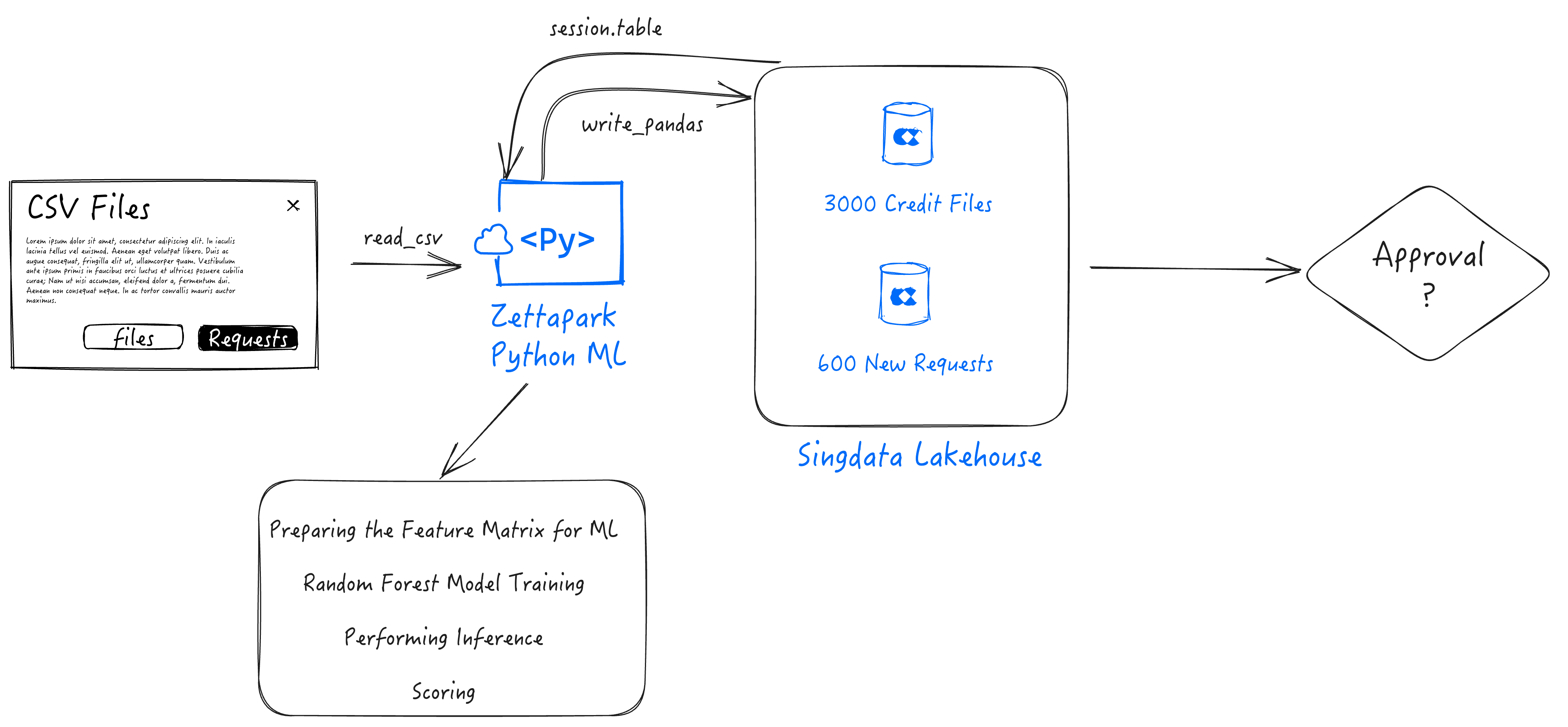
在本逐步教程中,您将能够使用适用于 Python 的 Zettapark,以及您最喜欢的数据分析和可视化 Python 库,以及流行的 scikit-learn 机器学习库,来解决一个端到端的机器学习用例。
:-: 
前提条件
- Lakehouse 账户
- 客户端 Zettapark 环境,已安装 Zettapark 库。
您将学到的内容
- 了解如何使用适用于 Python 的 Zettapark 实现端到端的机器学习管道。
- 使用适用于 Python 的 Zettapark API 和矢量化函数进行开发。
- 使用 Python 流行库(Pandas、seaborn)进行数据探索、可视化和准备。
- 使用 scikit-learn Python 包进行机器学习。
- 使用适用于 Python 的 Zettapark 部署和使用机器学习模型进行评分。
使用步骤
- 第 1 步:运行信用评分设置笔记本。这将下载数据集,并创建本演示所需的数据库和表。确保自定义 config.json。
- 第 2 步:现在您可以运行信用评分教程。
您可以从GitHub 存储库获取源代码(Jupyter Notebook ipynb 文件)和数据文件。
使用 Zettapark for Python 进行信用评分设置笔记本
1. Lakehouse 试用账户
先决条件是拥有一个 Lakehouse 账户。如果您没有 Lakehouse 账户,可以联系免费试用。
注册试用后,请收藏 Lakehouse 账户的 URL,并保存您的凭证,这些信息在本实验中需要使用。
此版本需要 Zettapark 0.1.2 或更高版本。
2. Python 库
运行此演示需要以下库。在此部分,添加环境中缺少的任何 Python 库。
# !pip install -q --upgrade clickzetta_zettapark_python
# !pip install scikit-plot
# !pip install pyarrow==6.0.0
# !pip install seaborn
# !pip install matplotlib
3. 文件下载
3.1 数据集
! curl -o data/credit_files.csv https://raw.githubusercontent.com/yunqiqiliang/clickzetta_quickstart/refs/heads/main/Zettapark-credit-scoring/data/credit_files.csv
  % Total    % Received % Xferd  Average Speed   Time    Time     Time  Current
                                 Dload  Upload   Total   Spent    Left  Speed
100  292k  100  292k    0     0  66280      0  0:00:04  0:00:04 --:--:-- 69100
! curl -o data/credit_request.csv https://raw.githubusercontent.com/yunqiqiliang/clickzetta_quickstart/refs/heads/main/Zettapark-credit-scoring/data/credit_request.csv
  % Total    % Received % Xferd  Average Speed   Time    Time     Time  Current
                                 Dload  Upload   Total   Spent    Left  Speed
100  6068  100  6068    0     0   2297      0  0:00:02  0:00:02 --:--:--  2297
3.2 config.json 凭证文件
需要编辑以下文件,填入 Lakehouse 账户的凭证并保存。它将用于在主笔记本中连接到 Lakehouse:
{
  "username": "<username>",
  "password": "<password>",
  "service": "<service url>",
  "instance": "<instance id>",
  "workspace": "<workspace>",
  "schema": "<schema>",
  "vcluster": "<vcluster>",
  "sdk_job_timeout": 60,
  "hints": {
    "sdk.job.timeout": 60,
    "query_tag": "test_zettapark_credit_scoring"
  }
}
! curl -o config/config_tobe_renamed.json https://raw.githubusercontent.com/yunqiqiliang/clickzetta_quickstart/refs/heads/main/Zettapark-credit-scoring/config/config.json
  % Total    % Received % Xferd  Average Speed   Time    Time     Time  Current
                                 Dload  Upload   Total   Spent    Left  Speed
100   321  100   321    0     0    138      0  0:00:02  0:00:02 --:--:--   138
4. 数据库
在下面的部分中,请在 config.json 文件中填写不同的参数,以连接到您的 Lakehouse 环境。
import pandas as pd
import json
from clickzetta.zettapark.session import Session
import clickzetta.zettapark.functions as F
import warnings

warnings.filterwarnings("ignore", category=FutureWarning)

# 从配置文件读取连接参数
with open('config/config.json', 'r') as config_file:
    config = json.load(config_file)

schema = config['schema']
vcluster = config['vcluster']

print("Connecting to Lakehouse.....\n")

# 创建会话
session = Session.builder.configs(config).create()

session.sql(f"CREATE SCHEMA IF NOT EXISTS {schema}").collect()
session.sql(f"CREATE VCLUSTER IF NOT EXISTS {vcluster} VCLUSTER_SIZE=1 VCLUSTER_TYPE = GENERAL").collect()

print(session.sql("SELECT current_instance_id(), current_workspace(),current_workspace_id(), current_schema(), current_user(),current_user_id(), current_vcluster()").collect())

print("\nConnected!...\n")
5. 表
此演示包含 2 张表:
-
CREDIT_FILES:此表包含当前文件上的信用情况以及贷款是否正在偿还或在偿还信用方面是否存在实际问题。此数据集将用于历史分析并构建机器学习模型,以对新申请进行评分。
-
CREDIT_REQUESTS:此表包含银行需要根据 ML 算法批准的新信用请求。
5.1 CREDIT_FILES 表
运行以下命令后,请登录到您的 Lakehouse 环境,确保表已创建。它应该有 2.9K 行。
credit_files = pd.read_csv('data/credit_files.csv')
credit_files.columns = credit_files.columns.str.lower()
session.sql("drop table if exists CREDIT_FILES").collect()
session.write_pandas(credit_files,"CREDIT_FILES",auto_create_table='True', quote_identifiers=False)
<clickzetta.zettapark.table.Table at 0x7fe58538e990>
credit_df = session.table("CREDIT_FILES")
credit_df.schema
StructType([StructField('`credit_request_id`', LongType(), nullable=True), StructField('`credit_amount`', LongType(), nullable=True), StructField('`credit_duration`', LongType(), nullable=True), StructField('`purpose`', StringType(), nullable=True), StructField('`installment_commitment`', LongType(), nullable=True), StructField('`other_parties`', StringType(), nullable=True), StructField('`credit_standing`', StringType(), nullable=True), StructField('`credit_score`', LongType(), nullable=True), StructField('`checking_balance`', DoubleType(), nullable=True), StructField('`savings_balance`', DoubleType(), nullable=True), StructField('`existing_credits`', LongType(), nullable=True), StructField('`assets`', StringType(), nullable=True), StructField('`housing`', StringType(), nullable=True), StructField('`qualification`', StringType(), nullable=True), StructField('`job_history`', LongType(), nullable=True), StructField('`age`', LongType(), nullable=True), StructField('`sex`', StringType(), nullable=True), StructField('`marital_status`', StringType(), nullable=True), StructField('`num_dependents`', LongType(), nullable=True), StructField('`residence_since`', LongType(), nullable=True), StructField('`other_payment_plans`', StringType(), nullable=True)])
credit_df.toPandas().head()
credit_df.toPandas().info()
<class 'pandas.core.frame.DataFrame'>
RangeIndex: 2940 entries, 0 to 2939
Data columns (total 21 columns):
 #   Column                  Non-Null Count  Dtype
---  ------                  --------------  -----
 0   credit_request_id       2940 non-null   int64
 1   credit_amount           2940 non-null   int64
 2   credit_duration         2940 non-null   int64
 3   purpose                 2940 non-null   object
 4   installment_commitment  2940 non-null   int64
 5   other_parties           271 non-null    object
 6   credit_standing         2940 non-null   object
 7   credit_score            2940 non-null   int64
 8   checking_balance        2940 non-null   float64
 9   savings_balance         2940 non-null   float64
 10  existing_credits        2940 non-null   int64
 11  assets                  2489 non-null   object
 12  housing                 2940 non-null   object
 13  qualification           2940 non-null   object
 14  job_history             2940 non-null   int64
 15  age                     2940 non-null   int64
 16  sex                     2940 non-null   object
 17  marital_status          2940 non-null   object
 18  num_dependents          2940 non-null   int64
 19  residence_since         2940 non-null   int64
 20  other_payment_plans     2940 non-null   object
dtypes: float64(2), int64(10), object(9)
memory usage: 482.5+ KB
5.2 CREDIT_REQUEST 表
运行以下命令后,请登录到您的 Lakehouse 环境,确保表已创建。它应该有 60 行。
credit_requests = pd.read_csv('data/credit_request.csv')
credit_requests.columns = credit_requests.columns.str.lower()
session.sql("drop table if exists CREDIT_REQUESTS").collect()
session.write_pandas(credit_requests,"CREDIT_REQUESTS",auto_create_table='True', quote_identifiers=False)
<clickzetta.zettapark.table.Table at 0x7fe50b7556d0>
credit_req_df = session.table("CREDIT_REQUESTS")
credit_req_df.schema
StructType([StructField('`credit_request_id`', LongType(), nullable=True), StructField('`credit_amount`', LongType(), nullable=True), StructField('`credit_duration`', LongType(), nullable=True), StructField('`purpose`', StringType(), nullable=True), StructField('`installment_commitment`', LongType(), nullable=True), StructField('`other_parties`', StringType(), nullable=True), StructField('`credit_score`', LongType(), nullable=True), StructField('`checking_balance`', DoubleType(), nullable=True), StructField('`savings_balance`', DoubleType(), nullable=True), StructField('`existing_credits`', LongType(), nullable=True), StructField('`assets`', StringType(), nullable=True), StructField('`housing`', StringType(), nullable=True), StructField('`qualification`', StringType(), nullable=True), StructField('`job_history`', LongType(), nullable=True), StructField('`age`', LongType(), nullable=True), StructField('`sex`', StringType(), nullable=True), StructField('`marital_status`', StringType(), nullable=True), StructField('`num_dependents`', LongType(), nullable=True), StructField('`residence_since`', LongType(), nullable=True), StructField('`other_payment_plans`', StringType(), nullable=True)])
credit_req_df.toPandas().head()
credit_req_df.toPandas().info()
<class 'pandas.core.frame.DataFrame'>
RangeIndex: 60 entries, 0 to 59
Data columns (total 20 columns):
 #   Column                  Non-Null Count  Dtype
---  ------                  --------------  -----
 0   credit_request_id       60 non-null     int64
 1   credit_amount           60 non-null     int64
 2   credit_duration         60 non-null     int64
 3   purpose                 60 non-null     object
 4   installment_commitment  60 non-null     int64
 5   other_parties           8 non-null      object
 6   credit_score            60 non-null     int64
 7   checking_balance        60 non-null     float64
 8   savings_balance         60 non-null     float64
 9   existing_credits        60 non-null     int64
 10  assets                  49 non-null     object
 11  housing                 60 non-null     object
 12  qualification           60 non-null     object
 13  job_history             60 non-null     int64
 14  age                     60 non-null     int64
 15  sex                     60 non-null     object
 16  marital_status          60 non-null     object
 17  num_dependents          60 non-null     int64
 18  residence_since         60 non-null     int64
 19  other_payment_plans     60 non-null     object
dtypes: float64(2), int64(10), object(8)
memory usage: 9.5+ KB
使用 Zeetapark for Python 进行信用评分
在此笔记本中,我们将使用 Zettapark Python API 进行信用卡评分演示。
在此场景中,Zettabank 希望利用其现有的信用文件来分析当前的信用状况,即贷款是否正在顺利偿还,或者是否存在任何延迟/违约情况。
基于当前的信用状况,Zettabank 希望基于数据集构建一个机器学习信用评分算法,以便能够自动评估贷款是否应该被批准或拒绝。
先决条件
请在运行此演示之前运行信用评分演示设置笔记本。
1. 数据探索
在此部分,我们将探索现有信用的数据集。
1.1 打开 Lakehouse 会话
import json


import pandas as pd
from clickzetta.zettapark import *
from clickzetta.zettapark.functions import *
# 从配置文件读取连接参数
with open('config/config.json', 'r') as config_file:
    config = json.load(config_file)


schema = config['schema']
vcluster = config['vcluster']


print("Connecting to Lakehouse.....\n")


# 创建会话
session = Session.builder.configs(config).create()


session.sql(f"CREATE SCHEMA IF NOT EXISTS {schema}").collect()
session.sql(f"CREATE VCLUSTER IF NOT EXISTS {vcluster} VCLUSTER_SIZE=1 VCLUSTER_TYPE = GENERAL").collect()


print(session.sql("SELECT current_instance_id(), current_workspace(),current_workspace_id(), current_schema(), current_user(),current_user_id(), current_vcluster()").collect())


print("\nConnected!...\n")
1.2 探索 Lakehouse 表中的数据
credit_df = session.table("CREDIT_FILES")
credit_df.describe().toPandas()
credit_df.toPandas().info()
<class 'pandas.core.frame.DataFrame'>
RangeIndex: 2940 entries, 0 to 2939
Data columns (total 21 columns):
 #   Column                  Non-Null Count  Dtype
---  ------                  --------------  -----
 0   credit_request_id       2940 non-null   int64
 1   credit_amount           2940 non-null   int64
 2   credit_duration         2940 non-null   int64
 3   purpose                 2940 non-null   object
 4   installment_commitment  2940 non-null   int64
 5   other_parties           271 non-null    object
 6   credit_standing         2940 non-null   object
 7   credit_score            2940 non-null   int64
 8   checking_balance        2940 non-null   float64
 9   savings_balance         2940 non-null   float64
 10  existing_credits        2940 non-null   int64
 11  assets                  2489 non-null   object
 12  housing                 2940 non-null   object
 13  qualification           2940 non-null   object
 14  job_history             2940 non-null   int64
 15  age                     2940 non-null   int64
 16  sex                     2940 non-null   object
 17  marital_status          2940 non-null   object
 18  num_dependents          2940 non-null   int64
 19  residence_since         2940 non-null   int64
 20  other_payment_plans     2940 non-null   object
dtypes: float64(2), int64(10), object(9)
memory usage: 482.5+ KB
credit_df.toPandas()
1.3 可视化数值特征
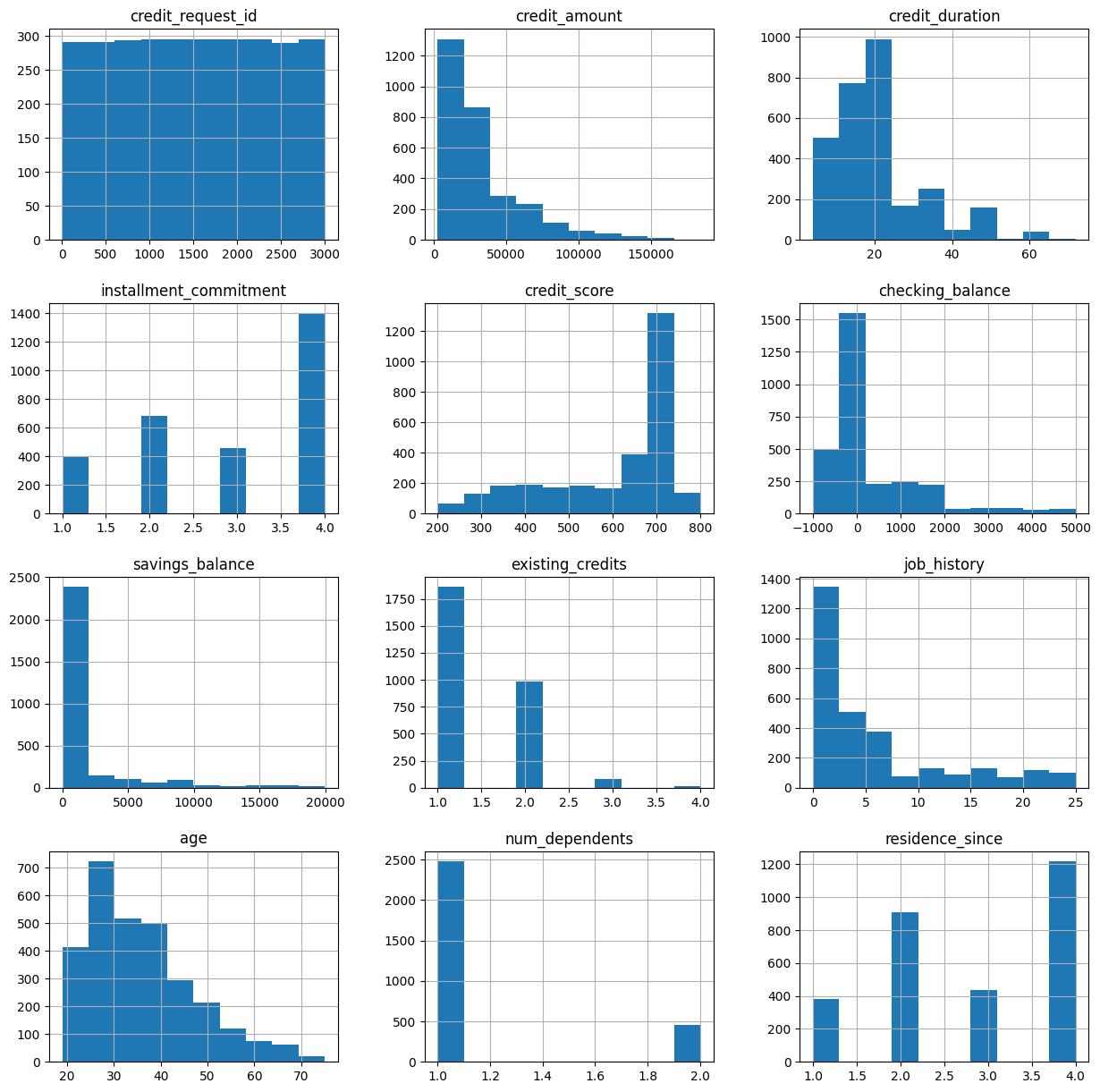
从这个可视化中,我们可以看到一些有趣的特征:
- 大多数信用请求的金额较小(<50k)
- 大多数信用期限为20个月或更短。
- 大多数申请人的信用评分很高。
- 大多数申请人在 Zettabank 的信贷或储蓄账户中余额不多。
- 大多数申请人年龄小于40岁。
credit_df.toPandas().hist(figsize=(15,15))
array([[<Axes: title={'center': 'credit_request_id'}>,
        <Axes: title={'center': 'credit_amount'}>,
        <Axes: title={'center': 'credit_duration'}>],
       [<Axes: title={'center': 'installment_commitment'}>,
        <Axes: title={'center': 'credit_score'}>,
        <Axes: title={'center': 'checking_balance'}>],
       [<Axes: title={'center': 'savings_balance'}>,
        <Axes: title={'center': 'existing_credits'}>,
        <Axes: title={'center': 'job_history'}>],
       [<Axes: title={'center': 'age'}>,
        <Axes: title={'center': 'num_dependents'}>,
        <Axes: title={'center': 'residence_since'}>]], dtype=object)
1.4 可视化分类特征
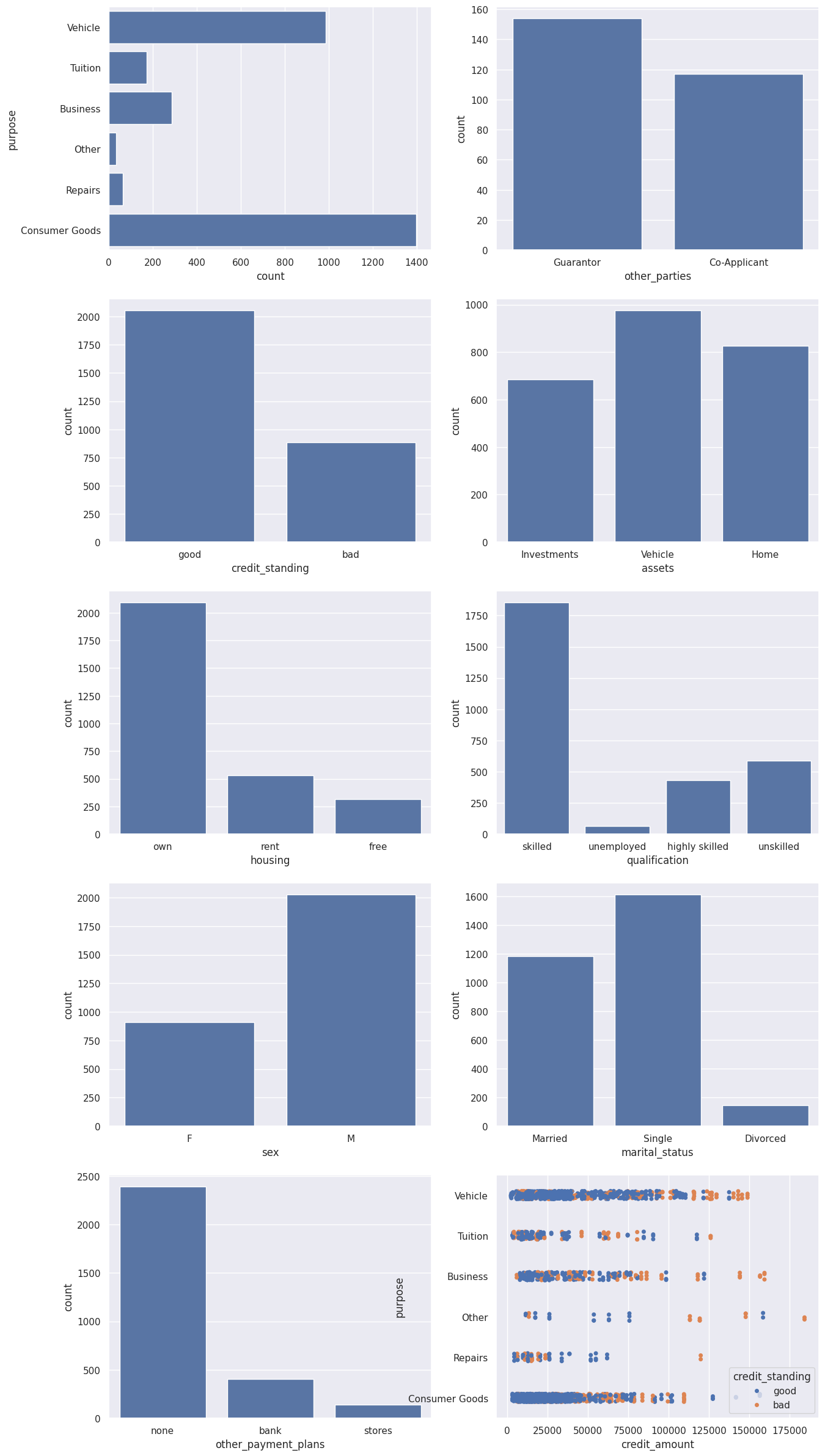
从这个可视化中,我们可以看到一些有趣的特征:
- 大多数流行的信用请求与车辆购买或消费品相关。
- 绝大多数贷款没有担保人,也没有共同申请人。
- 大多数文件中的信用状况良好。
- 大多数申请人是男性、外国工人、技术工人,拥有自己的房屋/公寓。
- 更高金额的贷款(每个贷款类别的阈值不同)有更高的违约可能性。
import matplotlib.pyplot as plt
import seaborn as sns


sns.set(style="darkgrid")


fig, axs = plt.subplots(5, 2, figsize=(15, 30))
df = credit_df.toPandas()
sns.countplot(data=df, y="purpose", ax=axs[0,0])
sns.countplot(data=df, x="other_parties", ax=axs[0,1])
sns.countplot(data=df, x="credit_standing", ax=axs[1,0])
sns.countplot(data=df, x="assets", ax=axs[1,1])
sns.countplot(data=df, x="housing", ax=axs[2,0])
sns.countplot(data=df, x="qualification", ax=axs[2,1])
sns.countplot(data=df, x="sex", ax=axs[3,0])
sns.countplot(data=df, x="marital_status", ax=axs[3,1])
sns.countplot(data=df, x="other_payment_plans", ax=axs[4,0])
sns.stripplot(y="purpose", x="credit_amount", data=df, hue='credit_standing', jitter=True, ax=axs[4,1])
plt.show()
1.5 通过 Zettapark API 运行查询
我们可以使用 Zettapark API 运行查询以获取各种见解。例如,让我们尝试确定不同类别的贷款范围。我们可以通过检查 Lakehouse 查询历史来了解 Zettapark API 如何作为 SQL 推送。
df_loan_status = credit_df.select(col("PURPOSE"),col("CREDIT_AMOUNT"))\
                          .groupBy(col("PURPOSE"))\
                          .agg([min(col("CREDIT_AMOUNT")).as_("MIN_CREDIT_AMOUNT"), max(col("CREDIT_AMOUNT")).as_("MAX_CREDIT_AMOUNT"), median(col("CREDIT_AMOUNT")).as_("MED_CREDIT_AMOUNT"),avg(col("CREDIT_AMOUNT")).as_("AVG_CREDIT_AMOUNT")])\
                          .sort(col("PURPOSE"))
df_loan_status.toPandas()
2. 数据转换和编码
对于当前用例,为了将数据准备成机器学习所需的格式,我们需要将分类值编码成数值。
为了实现这一点,我们可以利用 Zettapark Python API 进行编码。
2.1 准备机器学习的特征矩阵
在此部分,我们将利用 Zettapark Python API 准备一个随机森林分类器模型的特征矩阵。
from clickzetta.zettapark.functions import when


feature_matrix = credit_df.select(
    when(col("purpose") == "Consumer Goods", 1)
    .when(col("purpose") == "Vehicle", 2)
    .when(col("purpose") == "Tuition", 3)
    .when(col("purpose") == "Business", 4)
    .when(col("purpose") == "Repairs", 5)
    .otherwise(0).alias("purpose_code"),
    when(col("qualification") == "unskilled", 1)
    .when(col("qualification") == "skilled", 2)
    .when(col("qualification") == "highly skilled", 3)
    .otherwise(0).alias("qualification_code"),
    when(col("other_parties") == "Guarantor", 1)
    .when(col("other_parties") == "Co-Applicant", 2)
    .otherwise(0).alias("other_parties_code"),
    when(col("other_payment_plans") == "bank", 1)
    .when(col("other_payment_plans") == "stores", 2)
    .otherwise(0).alias("other_payment_plans_code"),
    when(col("housing") == "rent", 1)
    .when(col("housing") == "own", 2)
    .otherwise(0).alias("housing_code"),
    when(col("assets") == "Vehicle", 1)
    .when(col("assets") == "Investments", 2)
    .when(col("assets") == "Home", 3)
    .otherwise(0).alias("assets_code"),
    when(col("sex") == "M", 1)
    .otherwise(0).alias("sex_code"),
    when(col("marital_status") == "Married", 1)
    .when(col("marital_status") == "Single", 2)
    .otherwise(0).alias("marital_status_code"),
    when(col("credit_standing") == "good", 1)
    .otherwise(0).alias("credit_standing_code"),
    col("checking_balance"),
    col("savings_balance"),
    col("age"),
    col("job_history"),
    col("credit_score"),
    col("credit_duration"),
    col("credit_amount"),
    col("residence_since"),
    col("installment_commitment"),
    col("num_dependents"),
    col("existing_credits")
)


feature_matrix_pandas = feature_matrix.toPandas()
print(feature_matrix_pandas)
      purpose_code  qualification_code  other_parties_code  \
0                2                   2                   0
1                2                   2                   0
2                3                   2                   0
3                3                   2                   0
4                2                   2                   0
...            ...                 ...                 ...
2935             0                   0                   0
2936             2                   0                   0
2937             2                   0                   0
2938             2                   2                   0
2939             2                   2                   0


      other_payment_plans_code  housing_code  assets_code  sex_code  \
0                            0             2            0         0
1                            1             1            0         1
2                            0             1            2         0
3                            1             1            2         0
4                            0             2            2         0
...                        ...           ...          ...       ...
2935                         1             0            0         1
2936                         1             0            0         1
2937                         0             0            1         1
2938                         0             2            1         1
2939                         0             2            1         1


      marital_status_code  credit_standing_code  checking_balance  \
0                       1                     1           -728.12
1                       2                     1              0.00
2                       1                     1           4696.00
3                       1                     1            -25.35
4                       1                     1              0.00
...                   ...                   ...               ...
2935                    2                     1           1505.00
2936                    2                     1           4486.00
2937                    2                     1            720.00
2938                    2                     1            752.00
2939                    2                     1           1564.00


      savings_balance  age  job_history  credit_score  credit_duration  \
0               17.00   39           15           466                6
1             2443.00   35            1           202                6
2              143.00   23            1           736               15
3                0.00   23            3           732               12
4              510.00   30            1           507               18
...               ...  ...          ...           ...              ...
2935             0.00   40            0           726               48
2936          7361.86   66            0           343               12
2937           460.00   68            0           396               16
2938          1444.00   27            0           523               45
2939          1998.00   27            0           552               45


      credit_amount  residence_since  installment_commitment  num_dependents  \
0              8600                4                       1               1
1             12040                1                       4               1
2              3920                4                       4               1
3             12000                4                       4               1
4             10550                1                       4               1
...             ...              ...                     ...             ...
2935          53810                4                       3               1
2936          14800                4                       2               1
2937          11750                3                       2               1
2938          45760                4                       3               1
2939          45760                4                       3               1


      existing_credits
0                    2
1                    1
2                    1
3                    1
4                    2
...                ...
2935                 1
2936                 3
2937                 3
2938                 1
2939                 1


[2940 rows x 20 columns]
现在已定义了特征矩阵,我们将其转换为 Pandas DataFrame。
df = feature_matrix.toPandas().astype(int)
df.info()
<class 'pandas.core.frame.DataFrame'>
RangeIndex: 2940 entries, 0 to 2939
Data columns (total 20 columns):
 #   Column                    Non-Null Count  Dtype
---  ------                    --------------  -----
 0   purpose_code              2940 non-null   int64
 1   qualification_code        2940 non-null   int64
 2   other_parties_code        2940 non-null   int64
 3   other_payment_plans_code  2940 non-null   int64
 4   housing_code              2940 non-null   int64
 5   assets_code               2940 non-null   int64
 6   sex_code                  2940 non-null   int64
 7   marital_status_code       2940 non-null   int64
 8   credit_standing_code      2940 non-null   int64
 9   checking_balance          2940 non-null   int64
 10  savings_balance           2940 non-null   int64
 11  age                       2940 non-null   int64
 12  job_history               2940 non-null   int64
 13  credit_score              2940 non-null   int64
 14  credit_duration           2940 non-null   int64
 15  credit_amount             2940 non-null   int64
 16  residence_since           2940 non-null   int64
 17  installment_commitment    2940 non-null   int64
 18  num_dependents            2940 non-null   int64
 19  existing_credits          2940 non-null   int64
dtypes: int64(20)
memory usage: 459.5 KB
这是数据的样子:
df.head()
3. 随机森林模型训练
我们将使用 Python 中流行的 scikit-learn 机器学习库中的随机森林分类器模型。
from sklearn.model_selection import train_test_split


X_train, X_test, y_train, y_test = train_test_split(df.drop('credit_standing_code', axis=1),
                                                    df['credit_standing_code'], test_size=0.30)
from sklearn.ensemble import RandomForestClassifier


rfc = RandomForestClassifier(n_estimators=100)
rfc.fit(X_train, y_train)
4. 测试模型
rfc_pred = rfc.predict(X_test)
from sklearn.metrics import classification_report, confusion_matrix


print(classification_report(y_test,rfc_pred))
              precision    recall  f1-score   support


           0       0.99      0.87      0.92       275
           1       0.94      1.00      0.97       607


    accuracy                           0.96       882
   macro avg       0.97      0.93      0.95       882
weighted avg       0.96      0.96      0.95       882
print(confusion_matrix(y_test,rfc_pred))
[[238  37]
 [  2 605]]
5. 在 Lakehouse 中进行推理
在下面的例子中,我们希望处理 60 个待处理的信用请求,并对是否批准贷款进行评估。数据如下所示:
df_cred_req = session.table("CREDIT_REQUESTS")
df_cred_req.toPandas()
df.info()
<class 'pandas.core.frame.DataFrame'>
RangeIndex: 2940 entries, 0 to 2939
Data columns (total 20 columns):
 #   Column                    Non-Null Count  Dtype
---  ------                    --------------  -----
 0   purpose_code              2940 non-null   int64
 1   qualification_code        2940 non-null   int64
 2   other_parties_code        2940 non-null   int64
 3   other_payment_plans_code  2940 non-null   int64
 4   housing_code              2940 non-null   int64
 5   assets_code               2940 non-null   int64
 6   sex_code                  2940 non-null   int64
 7   marital_status_code       2940 non-null   int64
 8   credit_standing_code      2940 non-null   int64
 9   checking_balance          2940 non-null   int64
 10  savings_balance           2940 non-null   int64
 11  age                       2940 non-null   int64
 12  job_history               2940 non-null   int64
 13  credit_score              2940 non-null   int64
 14  credit_duration           2940 non-null   int64
 15  credit_amount             2940 non-null   int64
 16  residence_since           2940 non-null   int64
 17  installment_commitment    2940 non-null   int64
 18  num_dependents            2940 non-null   int64
 19  existing_credits          2940 non-null   int64
dtypes: int64(20)
memory usage: 459.5 KB
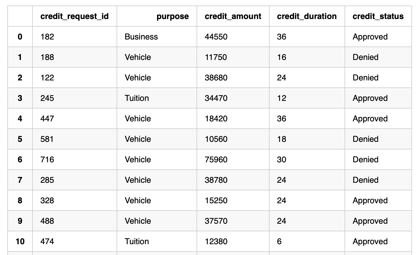
6. 开发评分函数
当 Zettabank 接收信用请求时,我们希望编写一个函数,该函数可以通过任务调用,对传入的微批请求进行评分。
Python 函数将首先使用 Zettapark API 构建模型的输入特征,以进行评分。
from clickzetta.zettapark.functions import col, when


def process_credit_requests_fn (session, credit_requests: str, credit_assessment: str) -> int:

    # 使用 Zettapark API 直接编码构建模型的输入特征。
    df_cred_req = session.table(credit_requests).select(
                            col("CREDIT_REQUEST_ID"), col("PURPOSE"),
                            when(col("PURPOSE") == "Consumer Goods", 1)
                            .when(col("PURPOSE") == "Vehicle", 2)
                            .when(col("PURPOSE") == "Tuition", 3)
                            .when(col("PURPOSE") == "Business", 4)
                            .when(col("PURPOSE") == "Repairs", 5)
                            .otherwise(0).alias("PURPOSE_CODE"),
                            when(col("QUALIFICATION") == "unskilled", 1)
                            .when(col("QUALIFICATION") == "skilled", 2)
                            .when(col("QUALIFICATION") == "highly skilled", 3)
                            .otherwise(0).alias("QUALIFICATION_CODE"),
                            when(col("OTHER_PARTIES") == "Guarantor", 1)
                            .when(col("OTHER_PARTIES") == "Co-Applicant", 2)
                            .otherwise(0).alias("OTHER_PARTIES_CODE"),
                            when(col("OTHER_PAYMENT_PLANS") == "bank", 1)
                            .when(col("OTHER_PAYMENT_PLANS") == "stores", 2)
                            .otherwise(0).alias("OTHER_PAYMENT_PLANS_CODE"),
                            when(col("HOUSING") == "rent", 1)
                            .when(col("HOUSING") == "own", 2)
                            .otherwise(0).alias("HOUSING_CODE"),
                            when(col("ASSETS") == "Vehicle", 1)
                            .when(col("ASSETS") == "Investments", 2)
                            .when(col("ASSETS") == "Home", 3)
                            .otherwise(0).alias("ASSETS_CODE"),
                            when(col("SEX") == "M", 1)
                            .otherwise(0).alias("SEX_CODE"),
                            when(col("MARITAL_STATUS") == "Married", 1)
                            .when(col("MARITAL_STATUS") == "Single", 2)
                            .otherwise(0).alias("MARITAL_STATUS_CODE"),
                            col("CHECKING_BALANCE"),
                            col("SAVINGS_BALANCE"),
                            col("AGE"),
                            col("JOB_HISTORY"),
                            col("CREDIT_SCORE"),
                            col("CREDIT_DURATION"),
                            col("CREDIT_AMOUNT"),
                            col("RESIDENCE_SINCE"),
                            col("INSTALLMENT_COMMITMENT"),
                            col("NUM_DEPENDENTS"),
                            col("EXISTING_CREDITS")
                         )

    # 调用 UDF 对之前读取的现有信用请求进行评分
    input_features = [ 'PURPOSE_CODE',
                   'QUALIFICATION_CODE',
                   'OTHER_PARTIES_CODE',
                   'OTHER_PAYMENT_PLANS_CODE',
                   'HOUSING_CODE',
                   'ASSETS_CODE',
                   'SEX_CODE',
                   'MARITAL_STATUS_CODE',
                   'CHECKING_BALANCE',
                   'SAVINGS_BALANCE',
                   'AGE',
                   'JOB_HISTORY',
                   'CREDIT_SCORE',
                   'CREDIT_DURATION',
                   'CREDIT_AMOUNT',
                   'RESIDENCE_SINCE',
                   'INSTALLMENT_COMMITMENT',
                   'NUM_DEPENDENTS',
                   'EXISTING_CREDITS']


    df_assessment = df_cred_req.select(
                    col("CREDIT_REQUEST_ID"), col("PURPOSE"), col("CREDIT_AMOUNT"), col("CREDIT_DURATION"),
                    when(col("CREDIT_SCORE") > 600, "Approved").otherwise("Denied").alias("CREDIT_STATUS"))

    df_assessment.write.mode("overwrite").saveAsTable(credit_assessment)

    # 函数将返回评估的信用请求数。
    return df_assessment.count()
7. 调用评分函数
process_credit_requests_fn (session, "credit_requests", "credit_assessments")
60
session.table("credit_assessments").toPandas()
附录: